The Inverse Variance Weighted Least Squares Simple Regression as Generalized Cochran–Armitage Test for Trend

Introduction

A trend test is a statistical method used to evaluate whether data across different groups follow a certain trend. One of the most well-known trend tests is the Cochran–Armitage test for trend, commonly referred to as the ${\chi }^2$ test for trend, which is applied to 2 × $k$ contingency tables when the $k$ groups have an ordinal relationship.1–3 Others are the Jonckheere–Terpstra and Cuzick’s tests, which are applied to non-parametric individual data with an ordinal structure.4–6 These trend tests can be applied to various types of ordered data, such as time since drug administration, drug dosage, patient age groups, genotypes, and disease severity levels. In sociological and psychological studies, variables such as income, educational attainment, and developmental level can also be treated as ordinal variables across groups. Although these trend tests are powerful tools, their need for specific data formats limits their applicability. Many researchers have sought a more versatile trend test that can be applied more broadly.

A related issue concerning data types has been discussed in the context of meta-analysis. Conventional meta-analyses using the Peto and Mantel–Haenszel methods combine risk ratios, odds ratios, and risk differences, all of which require 2 × 2 contingency tables.7–9 In meta-analyses, detailed raw data from published studies are often unavailable, even though summary estimates of key statistics, such as odds ratios and their 95% confidence intervals, are easily accessible. The inverse variance method, which applies inverse variance weighting, enables data integration without requiring detailed raw data. Moreover, the inverse variance method can handle data formats that the Peto and Mantel–Haenszel methods cannot, such as adjusted odds ratios from multivariate analyses and hazard ratios. The incorporation of inverse variance weighting has greatly expanded the scope of meta-analysis and significantly accelerated research across almost all areas of clinical medicine.10–12

This article demonstrates that the inverse variance weighted least squares simple regression model generalizes the Cochran–Armitage test for trend, although this concept has not been widely recognized. This method allows for trend testing within ordered groups even without access to detailed individual data, as long as summary statistics or effect measures, along with variance, are available. For clarity, we propose naming this test as the ‘Inverse Variance Trend Test’ or the ‘Generalized Cochran–Armitage Test.’ Following the theoretical explanation, we demonstrate the wide applicability of this test across a variety of datasets by applying it to five medical case examples.

Methods

Definition of the Inverse Variance Trend Test

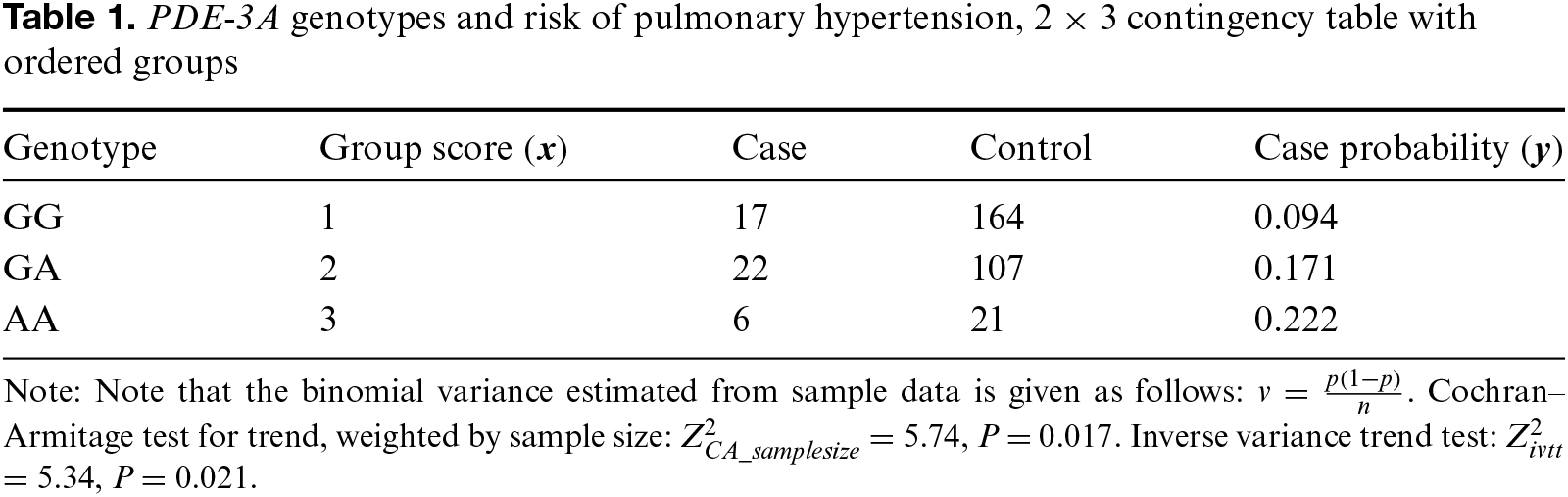
We assume that k-ordered groups have continuous dependent variables y, where the intervals between values are consistent. Each $y_i$ has the estimated variance $v_i$ (Table 1). The groups are assigned a group score $x$. As in the Cochran–Armitage test, it is standard to assign natural numbers $x$ starting from 1 to the groups, but in cases of ties, the average value is assigned. If clear numerical values exist for each group, such as drug dosages, these can be used for the group scores. In inverse variance weighting, the weight ($w$) of each group is defined by the inverse of the estimated variance of $y$, $w_i=\frac{1}{v_i}$.10–12 It is assumed that the error terms in the regression analysis follow a normal distribution, and the sample size should be sufficiently large for the central limit theorem to apply. The data format for the trend test is shown in Table S1.

In weighted least squares univariate regression analysis, the slope ($\hat{\beta }$) and its standard error (SE($\hat{\beta }$)) are given as follows (Fig. S1)13–15:

$$\hat{\beta }=\frac{\sum _{i=1}^k{w}_i(y_i-\overline{y})(x_i-\overline{x})}{\sum _{i=1}^k{w}_i(x_i-\overline{x}{)}^2},$$

$$\left(\text{SE}\left(\hat{\beta }\right)\right)=\frac{1}{\sqrt{}\sum _{i=1}^k{w}_i{(x_i-\overline{x})}^2}$$

Here, we define the Z score for the inverse variance trend test ($Z_{ivtt}$) as follows:

$$Z_{ivtt}=\frac{\hat{\beta }}{\text{SE}(\beta )}=\frac{\sum _{i=1}^k{w}_i(y_i-\overline{y})(x_i-\overline{x})}{\sqrt{}\sum _{i=1}^k{w}_i(x_i-\overline{x}{)}^2}\sim \text{N}(0,1)$$

$$Z_{ivtt}^2=\frac{[\sum _{i=1}^k{w}_i(y_i-\overline{y})(x_i-\overline{x}){]}^2}{\sum _{i=1}^k{w}_i(x_i-\overline{x}{)}^2}=\frac{[\sum _{i=1}^k\frac{1}{v_i}(y_i-\overline{y})(x_i-\overline{x}){]}^2}{\sum _{i=1}^k\frac{1}{v_i}(x_i-\overline{x}{)}^2}\sim {\chi }^2(\text{df }=1)$$

The null hypothesis is that 𝑦 is independent from 𝑥, or $\hat{\beta }$ = 0.

As we adopted inverse variance weighting, the averages, $\overline{x}$ and $\overline{y}$, are calculated as follows:

$$\overline{x}=\frac{\sum _{i=1}^k{w}_i{x}_i}{\sum _{i=1}^k{w}_i}=\frac{\sum _{i=1}^k\frac{1}{v_i}{x}_i}{\sum _{i=1}^k\frac{1}{v_i}}$$

$$\overline{y}=\frac{\sum _{i=1}^k{w}_i{y}_i}{\sum _{i=1}^k{w}_i}=\frac{\sum _{i=1}^k\frac{1}{v_i}{y}_i}{\sum _{i=1}^k\frac{1}{v_i}}$$

We can interpret $\overline{y}$ as the pooled value from a fixed-effect model meta-analysis (Fig. 1). Similarly, $\overline{x}$ can be recognized as the pooled value from a fixed-effect model meta-analysis weighted by the inverse variance of $y$ (Fig. S1).

Figure 1. PD-L1 expression level and hazard ratio for event-free survival, hazard ratios for ordered groups. Error bars indicate 95% confidence interval (95% CI). Note that y = log (hazard ratio) and v = log (95% CI upper · limit/95%CI lower limit) . Inverse variance trend test: Z2ivtt = 5.25, P = 2 1.96 0.022.

In general, fixed-effect model meta-analysis requires the absence of heterogeneity among groups. However, the goal here is not to obtain a pooled value but to demonstrate that the result of the calculation coincides with that of a fixed-effect model meta-analysis. Therefore, heterogeneity among the groups is not a concern.

Generalization from Cochran–Armitage test for trend

The following Z score represents one of the standard formulas for the Cochran–Armitage test for trend, weighted by sample size ($Z_{CA\mathrm{\_}samplesize}$).16,17

$$Z_{CA\mathrm{\_}samplesize}^2=\frac{[\sum _{i=1}^k{n}_i(p_i-p)(x_i-\overline{x}){]}^2}{p(1-p)\sum _{i=1}^k{n}_i(x_i-\overline{x}{)}^2}.$$

By dividing both the numerator and the denominator of this equation by $p(1-p)$ twice, we obtain the following equation:

$$Z_{CA\mathrm{\_}samplesize}^2=\frac{[\sum _{i=1}^k{\displaystyle \frac{n_i}{p(1-p)}}(p_i-p)(x_i-\overline{x}){]}^2}{\sum _{i=1}^k{\displaystyle \frac{n_i}{p(1-p)}}(x_i-\overline{x}{)}^2}.$$

Considering that the variance of a proportion is generally given by $\frac{p(1-p)}{n}$ and $w$ = $\frac{n}{p(1-p)}$, once we assume $p_i$ $\approx$ $p$, $Z_{CA\mathrm{\_}samplesize}^2$ can be rewritten as:

The Cochran–Armitage test can be defined by the following formula:

$$Z_{CA\mathrm{\_}samplesize}^2\approx \frac{{\left[\sum _{i=1}^k{\displaystyle \frac{n_i}{p_i(1-p_i)}}(p_i-p)(x_i-\overline{x})\right]}^2}{\sum _{i=1}^k{\displaystyle \frac{n_i}{p_i(1-p_i)}}{(x_i-\overline{x})}^2}=\frac{{\left[\sum _{i=1}^k{w}_i(p_i-p)(x_i-\overline{x})\right]}^2}{\sum _{i=1}^k{w}_i{(x_i-\overline{x})}^2}.$$

There have been variations in the weighting per group in the Cochran–Armitage test from its conception. While weighting based on only event counts (e.g., success or failure) was historically preferred,1–3 observation counts (e.g., the sum of successes and failures) have been more commonly used in recent years.16,17 Besides, weighting by inverse variance can also be justified.10–12 In this context, the Z score for the Cochran–Armitage test for trend with inverse variance weighting ($Z_{CA\mathrm{\_}ivw}$) is directly derived:

$$Z_{CA\mathrm{\_}ivw}^2=\frac{{\left[\sum _{i=1}^k{w}_i(p_i-p)(x_i-\overline{x})\right]}^2}{\sum _{i=1}^k{w}_i{(x_i-\overline{x})}^2}=\frac{{\left[\sum _{i=1}^k{\displaystyle \frac{1}{v_i}}(p_i-p)(x_i-\overline{x})\right]}^2}{\sum _{i=1}^k{\displaystyle \frac{1}{v_i}}{(x_i-\overline{x})}^2}\sim {\chi }^2(df=1).$$

By replacing the proportion $p$ with the continuous variable $y$, this formula becomes identical to $Z_{ivtt}^2$. Therefore, the test for the slope of weighted least squares univariate regression analysis can be considered generalized to the Cochran–Armitage test.

Examples

The five examples were selected for educational purposes to help readers understand the inverse variance trend test and apply it to real data.

Example 1

Table 1 summarizes a case–control study investigating whether the PDE-3A (rs10770682) genotype is associated with the risk of persistent pulmonary hypertension in newborns.18 At the rs10770682 locus, G is the major allele and A is the minor allele. The possible genotypic combinations—GG, GA, and AA—therefore form an ordered sequence (Table 1). As is conventional, group scores were assigned as 1, 2, and 3. Alternatively, the number of minor alleles (0, 1, and 2) could be used without affecting the test results. The result from the inverse variance trend test suggested significance ($Z_{ivtt}^2$ = 5.34, $P$ = 0.021). This result closely approximates that obtained from the traditional Cochran–Armitage test for trend, weighted by sample size ($Z_{CA\mathrm{\_}samplesize}^2$ = 5.74, $P$ = 0.017).

Example 2

In a multicenter trial, 796 patients with metastatic castration-resistant prostate cancer were randomized into olaparib and placebo arms.19 After two patients were removed for various reasons, 794 were evaluated for adverse events. Patients with and without grade 3 or higher adverse events are summarized in Table 2.

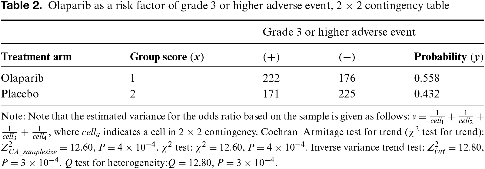
Although a trend test is usually not applied to a 2 × 2 contingency table, applying it here can help in understanding relevant tests (Table S2). The Cochran–Armitage test for trend weighted by sample size, which is also referred to as ${\chi }^2$ test for trend leads to the same result as the regular ${\chi }^2$ test for a 2 $\times$ 2 contingency table (${\chi }^2$ = $Z_{CA\mathrm{\_}samplesize}^2$ = 12.60). Similarly, inverse variance trend test and $Q$ test for heterogeneity yield the same results ($Z_{ivtt}^2$ = $Q$ = 12.80). In the comparison between the two groups, the $Q$ statistic and $Z_{ivtt}^2$ are calculated based on the same formula, and both evaluate the difference in group means adjusted by the inverse variance-weighted standard error. Therefore, these two tests can be considered equivalent.

Example 3

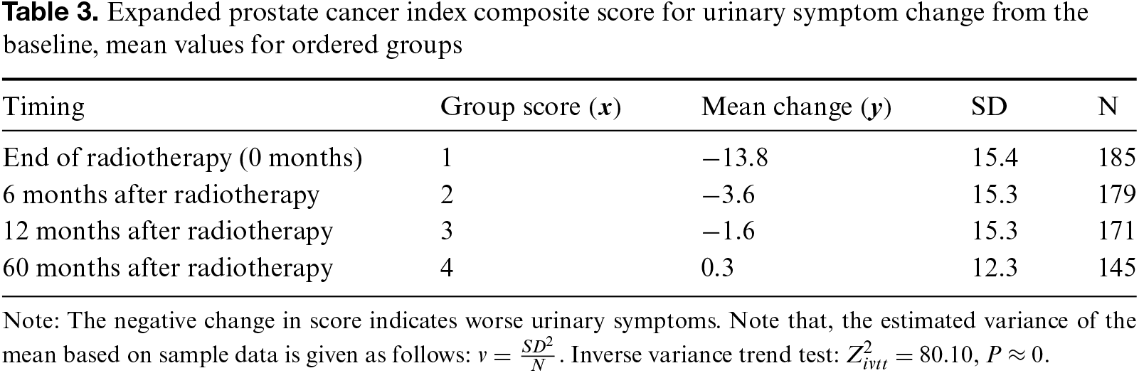
Patients with intermediate-risk prostate cancer enrolled in a randomized trial. Out of 420 patients, we extracted data from 205 patients who were treated with combined radiotherapy and total androgen suppression therapy.20 The Expanded Prostate Cancer Index Composite scoring system was used for quality-of-life assessment, as shown in Table 3. Although the inverse variance trend test can directly adopt the follow-up duration of 0 to 60 months as the explanatory variable $x$, some may hesitate to do so because 60 months might appear as an outlier compared to 0, 6, and 12 months. In such a case, the Jonckheere–Terpstra test for trend is a traditional choice, treating the Expanded Prostate Cancer Index Composite score as non-parametric. However, the individual data were consolidated during aggregation into mean, standard deviation (SD), and patient numbers (N), as shown in Table S2. If desired, 0, 6, 12, and 60 can be adoptable for group scores for the inverse variance trend test. However, the group’s scores from 1 to 4 were assigned. The results of the test indicate that the improvement in the scores over time is unlikely to be due to chance ($Z_{ivtt}^2$ = 80.10, $P$ $\approx$ 0).

Example 4

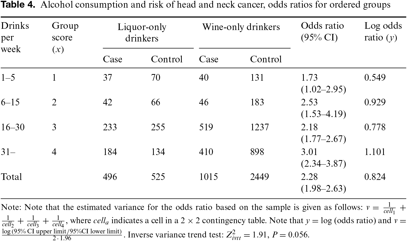
A pooled analysis of data from 15 case–control studies examined the association between the type of alcoholic beverage and the risk of head and neck cancer.21 In the ‘Total’ row of Table 4, it is evident that liquor-only drinkers have a higher risk of head and neck cancer compared to wine-only drinkers, with an odds ratio of 2.28. The same trend is observed when stratifying by the number of drinks per week. Among subjects who drink five or fewer drinks per week, liquor-only drinkers have a higher cancer risk than the corresponding wine-only drinkers, with an odds ratio of 1.73. In the subgroup of those who drink 31 or more drinks per week, the odds ratio increases to 3.01. Our primary interest lies in whether the odds ratio between liquor-only and wine-only drinkers changes as weekly alcohol consumption increases. This could be interpreted as an interaction between the type of alcohol and the cancer risk, with alcohol consumption acting as a potential effect modifier. However, the inverse variance trend test did not indicate a statistically significant interaction ($Z_{ivtt}^2$ = 1.91, $P$ = 0.056).

Example 5

A phase 3 trial randomized 397 patients with early-stage non-small-cell lung cancer to receive either pembrolizumab or placebo, with the primary endpoint being the hazard ratio for event-free survival.22 This medication is generally more effective for patients with higher PD-L1 expression levels, and visual inspection of Fig. 1 suggests that this trend may also apply in this study. It is customary to use 1% and 50% as cut-off values for PD-L1. These distinctive cut-offs make us hesitant to use the PD-L1 expression rate itself as an explanatory variable, prompting us to treat the three groups as an ordinal variable instead. The significance observed in the inverse variance trend test ($Z_{ivtt}^2$ = 5.25, $P$ = 0.022, Fig. 1) supports this trend.

Discussion

We have developed the inverse variance trend test integrating least squares simple regression analysis and inverse variance weighting to provide a versatile trend testing approach applicable in various scenarios. This test works as a generalized version of the Cochran–Armitage test for trends. It also yields consistent results with the Cochrane $Q$ test for meta-analysis when there are only two groups. The concept of trend testing began in the early 20th century, particularly in biology and medical research, to analyze ordered categorical data, such as genotype and medication dosage. William Cochran and Peter Armitage developed the trend test in the 1950s for ordered 2 × $k$ contingency tables, which is later referred to as the Cochran–Armitage test for trend.1–3 Jonckheere–Terpstra test and Cuzick’s test are other trend tests for ordinal data. With the advancement and widespread adoption of statistical software during the 1980s and 1990s, these tests for trends became widely used. Recently, these tests have played a crucial role in evidence-based medical research. They uncover patterns and trends in data, yielding vital scientific insights. However, the Cochran–Armitage test could not be applied to data format other than 2 × $k$ contingency tables. Similarly, the Jonckheere–Terpstra and Cuzick’s tests are only applicable when individual values are available.

Inverse variance weighting, a prevalent method in statistics, particularly in meta-analysis, operates on the principle that the smaller the variance of a dataset, the greater its weight in the analysis.10–12 In contrast, studies with larger variances, indicating higher uncertainty, have less impact on the overall outcomes in meta-analyses. Inverse variance weighting can be applied across a variety of statistical values, such as probability, mean difference, odds ratio, and hazard ratio, making it a highly adaptable statistical method. The proposed inverse variance trend test stems from the Cochran–Armitage test but has significantly broader applicability. The development of this flexible trend test is expected to enhance the quality of research and foster new scientific discoveries.

Our proposed inverse variance trend test utilizes a simple regression model, but it may be possible to apply a similar approach in a multiple regression framework.23–25 Expanding the current model to include multiple independent variables would allow for trend analysis while adjusting for the effects of other factors and covariates. Although this falls beyond the scope of our present manuscript, we hope future researchers will establish a trend test within a multiple regression model.

One limitation of the inverse variance trend test is its inapplicability in cases where neither variance, standard deviations, standard errors, nor 95% confidence intervals are available. Additionally, the applicability of the inverse variance trend test may be limited due to the normality requirement for the dependent variable $y$. For example, if the dependent variable is a strongly skewed serum C-reactive protein level, the inverse variance trend test may not be applicable. However, similar to many statistical methods that assume normality, it is often possible to obtain acceptable normality by log-transforming the dependent variable. Another limitation is the lack of robustness when the sample size is small or data are skewed. Furthermore, the inverse variance trend test requires interval-scale data and is not applicable to ordinal data. When individual ordinal data are provided, Cuzick’s test should be used instead. We hope the Excel file in the Supplementary Material will support readers in their analyses (Supplementary Excel file).

Conclusion

We demonstrated that the inverse variance weighted least squares simple regression model, functioning as the generalized Cochran–Armitage test for trend, is a highly versatile trend testing tool. When both the Cochran–Armitage and newly proposed tests can be applied, their test results are nearly identical. Additionally, the newly proposed test offers a significant advantage in enabling trend testing even when individual data are unavailable. This trend test is expected to enhance research in medicine and other fields.

Acknowledgment

None.

Funding Source

None.

Author contributions

N Horita contributed to the conception, data acquisition, analysis, interpretation, drafting, revision, final approval, and accountability. T. Mihara, Y. Mizuki, and T. Kawagoe contributed to the revision, final approval, and accountability.

Data availability Statement

Not applicable.

Ethical Statement

Not applicable.

Conflicts of Interest

The authors have nothing to declare.

Supplemental Information

Supplemental information for this article can be found online at https://sup.jclinque.com/api/articles/51/download-suppl.

References

1. Cochran WG. Some methods for strengthening the common χ2 tests. Bioethics. 1954;10(4):417–451. doi:10.2307/3001616.

2. Armitage P. Tests for linear trends in proportions and frequencies. Biometrics. 1955;11(3):375–386. doi:10.2307/3001775.

3. Tekindal MA, Güllü Ö., Yazici AC, et al. The estimating sample size for trend analysis of proportions in biological data using the cochran-armitage test. Turk J Field Crops. 2016;21(2):286–297. doi:10.17557/tjfc.33765.

4. Vock M, Balakrishnan N. A Jonckheere-Terpstra-type test for perfect ranking in balanced ranked set sampling. J Stat Plann Inference. February 2011;141(2):624–630. doi:10.1016/j.jspi.2010.07.005.

5. Terpstra TJ. The asymptotic normality and consistency of kendall’s test against trend, when ties are present in one ranking. Indagationes Mathematicae (Proceedings). January 1, 1952;55(2):327–333. doi:10.1016/S1385-7258(52)50043-X.

6. Jonckheere AR. A distribution-free k-sample test against ordered alternatives. Biometrika. 1954;1(2)):133–145. doi:10.2307/2333011.

7. Berlin JA, Laird NM, Sacks HS, Chalmers TC. A comparison of statistical methods for combining event rates from clinical trials. Stat Med. February 1989;8(2):141–151. doi:10.1002/sim.4780080202.

8. Viechtbauer W. Conducting meta-analyses in R with the metafor package. J Stat Softw. August 2010;36(3):1–48. doi:10.18637/jss.v036.i03.

9. Deeks JJ, Higgins JP, Altman DG. Meta-analysis of dichotomous outcomes. Publishen 2024. Accessed November 14, 2024. https://training.cochrane.org/handbook/current/chapter-10#section-10-4.

10. Sanchez-Meca J, Marin-Martinez F. Weighting by inverse variance or by sample size in meta-analysis: a simulation study. Educ Psychol Meas. April 1998;58(2):211–220. doi:10.1177/0013164498058002005.

11. Marín-Martínez F, Sánchez-Meca J. Weighting by inverse variance or by sample size in random-effects meta-analysis. Educ Psychol Meas. February 2010;70(1):56–73. doi:10.1177/0013164409344534.

12. Deeks JJ, Higgins JP, Altman DG. A generic inverse-variance approach to meta-analysis. Publishen 2024. Accessed on Nov 14, 2024. https://training.cochrane.org/handbook/archive/v6/chapter-10#section-10-3.

13. Rosner B. Fundamentals of Biostatistics. 8th ed. Brooks/Cole Publishing Company; 2015.

14. Canty AJ. Applied regression analysis with SAS. Published 2019. Accessed November 13, 2024. https://www.math.mcmaster.ca/canty/teaching/stat3a03/Lectures1.pdf.

15. Ruppert D, Wand MP. Multivariate locally weighted least squares regression. Ann Stat. 1994;22(3):1346–1370. doi:10.1214/aos/1176325632.

16. Liu H. Cochran-Armitage trend test using SAS. Published 2007. Accessed on November 15, 2024. https://www.lexjansen.com/pharmasug/2007/sp/SP05pdf.

17. Agresti A. Categorical Data Analysis. 3rd ed. Wiley; 2012.

18. Nakwan N, Mahasirimongkol S, Satproedprai N, et al. Possible association between a polymorphism of EPAS1 gene and persistent pulmonary hypertension of the newborn: a case-control study. J Pediatr (Rio J). July–August 2022;98(4):383–389. doi:10.1016/j.jped.2021.09.003.

19. Saad F, Clarke NW, Oya M, et al. Olaparib plus abiraterone versus placebo plus abiraterone in metastatic castration-resistant prostate cancer (PROpelfinal prespecified overall survival results of a randomised, double-blind, phase 3 trial. Lancet Oncol. October 2023;24(10):1094–1108. doi:10.1016/S1470-2045(23)00382-0.

20. Movsas B, Rodgers JP, Elshaikh MA, et al. Dose-escalated radiation alone or in combination with short-term total androgen suppression for intermediate-risk prostate cancer: patient-reported outcomes from NRG/radiation therapy oncology group 0815 randomized trial. J Clin Oncol. June 2023;10(17):3217–3224. doi:10.1200/JCO.22.02389.

21. Purdue MP, Hashibe M, Berthiller J, et al. Type of alcoholic beverage and risk of head and neck cancer–a pooled analysis within the INHANCE Consortium. Am J Epidemiol. January 15, 2009;169(2):132–142. doi:10.1093/aje/kwn306.

22. Wakelee H, Liberman M, Kato T, et al. Perioperative pembrolizumab for early-stage non-small-cell lung cancer. N Engl J Med. August 2023;10(6):491–503. doi:10.1056/NEJMoa2302983.

23. Roustaei N. Application and interpretation of linear-regression analysis. Med Hypothesis Discov Innov Ophthalmol. Fall 2024;13(3):151–159. doi:10.51329/mehdiophthal1506.

24. Toothaker LE. Multiple regression: testing and interpreting interactions. J Oper Res Soc. 1994;45(1):119–120. doi:10.1057/jors.1994.16.

25. Preacher KJ, Curran PJ, Bauer DJ. Computational tools for probing interactions in multiple linear regression, multilevel modeling, and latent curve analysis. J Educ Behav Stat. 2006;31(4):437–448. doi:10.3102/10769986031004437.

Copyright: © 2024 Horita et al. This work is licensed under a Creative Commons Attribution 4.0 International License, which permits unrestricted use, distribution, and reproduction in any medium, provided the original work is properly cited.